AzureDeveloper

Jupyter for Azure机器学习五天入门 - Day2 使用Jupyter训练图像分类的模型

分类: Azure机器学习 ◆ 标签: #Azure #人工智能 #机器学习 #JupyterBook ◆ 发布于: 2023-06-11 21:48:53

我们在前面Python的教程中我们也训练了模型，在之前的教程中我们直接使用了python脚本进行训练，我们这个系列向大家介绍更好用的工具jupyter, 给大家介绍如何使用jupyter book结合Azure Machine Learning进行机器学习项目的开发，在开始这个教程之前，建议大家先熟悉之前的一系列的教程，同时必须熟悉环境的搭建，环境搭建参考下述两篇文章:

创建Azure机器学习的本地环境和云环境
 准备Jupyter Book环境 Azure机器学习

另外我们前面的python的教程主要向大家介绍：

云环境和本地环境的构建
Python SDK的基本使用。
Python 训练脚本的编写
向Azure Machine Learning提交训练
介绍Azure Machine Learning基本的元素和基本概念，我们后面也会进一步的加深这个部分的学习。

那么在Jupyter一些类的教程中，我们主要讨论这些主题:

使用jupyter和Azure Machine Learning结合训练模型，注册模型，监控训练过程。
注册训练成功的模型，部署模型，使用rest api测试模型。
使用pipeline进行自动模型训练。

本节说明

我们在本节主要使用线性回归的算法对来自opendataset的MNIST数据集，同时使用scikit-learn框架进行模型训练。同时也需要注意一点是我们这里使用jupyter在Azure Machine Learning上进行远程训练。

设置环境

已经设置好conda环境之后，可以使用conda激活已经创建的环境

conda activate myml

为了运行本章的案例，还需要安装一些必须的包:

pip install azureml-sdk[notebooks] azureml-opendatasets matplotlib

然后请保证你本地的jupyter notebook已经启动，并且已经在Azure上创建好了Azure Machine Learning的资源，同时也下载了config.js，并放置在你项目的根目录。

在项目的根目录中启动jupyter, 然后打开浏览器访问jupyter notebook

jupyter notebook

新建一个book, 注意Python的环境选择您上一章设定的conda的环境，例如我的机器上是Python(MyML)

至此环境设定好了。我们开始继续下一步。

开始`Jupyter notebook`项目

我们现在开始本节的培训。

本章`jupyter notebook` 源码

您可以直接从下述位置查看文章的源码:
https://github.com/hylinux/azure-demo/blob/main/azure-machine-learning/jupyter-5-days/Day-1.ipynb

导入我们需要的包

在jupyter notebook里导入包

%matplotlib inline
import numpy as np
import matplotlib.pyplot as plt

import azureml.core
from azureml.core import Workspace

# check core SDK version number
print("Azure ML SDK Version: ", azureml.core.VERSION)

如下图:

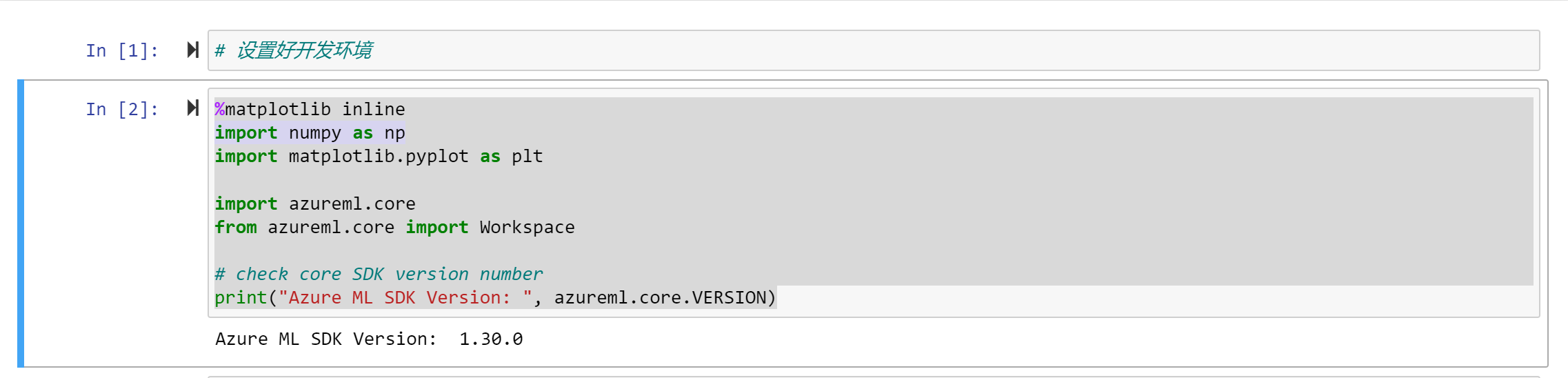
这之后不再截图了，大家可以自己打开jupyter book文件来看看。

链接到workspace

链接之前，请确保下载了config.js以及设置了Azure Cli到您想操作的云环境

ws = Workspace.from_config()
print(ws.name, ws.location, ws.resource_group, sep='\t')

创建一个`experiment`

我们之前也讨论过experiment, 每个运行都必须和一个experiment相关联。使用如下的代码进行创建:

from azureml.core import Experiment
experiment_name = 'Tutorial-sklearn-mnist'

exp = Experiment(workspace=ws, name=experiment_name)

创建或者attach一个计算实例(集群)

我们所有的训练操作都是需要计算资源的，这里我们是一个计算集群用于计算资源。我们的计算资源分成两类:

computer instance
computer cluster

另外根据CPU不同也分为基于CPU和基于GPU的，如果你需要创建基于GPU的资源，一定要注意自己是否有足够多的quota

from azureml.core.compute import AmlCompute
from azureml.core.compute import ComputeTarget
import os

# choose a name for your cluster
compute_name = os.environ.get("AML_COMPUTE_CLUSTER_NAME", "cpu-cluster")
compute_min_nodes = os.environ.get("AML_COMPUTE_CLUSTER_MIN_NODES", 0)
compute_max_nodes = os.environ.get("AML_COMPUTE_CLUSTER_MAX_NODES", 4)

# This example uses CPU VM. For using GPU VM, set SKU to STANDARD_NC6
vm_size = os.environ.get("AML_COMPUTE_CLUSTER_SKU", "STANDARD_D2_V2")


if compute_name in ws.compute_targets:
    compute_target = ws.compute_targets[compute_name]
    if compute_target and type(compute_target) is AmlCompute:
        print('found compute target. just use it. ' + compute_name)
else:
    print('creating a new compute target...')
    provisioning_config = AmlCompute.provisioning_configuration(vm_size=vm_size,
                                                                min_nodes=compute_min_nodes,
                                                                max_nodes=compute_max_nodes)

    # create the cluster
    compute_target = ComputeTarget.create(
        ws, compute_name, provisioning_config)

    # can poll for a minimum number of nodes and for a specific timeout.
    # if no min node count is provided it will use the scale settings for the cluster
    compute_target.wait_for_completion(
        show_output=True, min_node_count=None, timeout_in_minutes=20)

    # For a more detailed view of current AmlCompute status, use get_status()
    print(compute_target.get_status().serialize())

数据处理

我们在本节要使用到的数据是从MNIST开放数据集中来的，如果要使用这个数据我们需要先将该数据下载回来，然后解压，做一定的预处理。

下载数据

我们继续使用python脚本来下载数据

from azureml.core import Dataset
from azureml.opendatasets import MNIST

data_folder = os.path.join(os.getcwd(), 'data')
os.makedirs(data_folder, exist_ok=True)

mnist_file_dataset = MNIST.get_file_dataset()
mnist_file_dataset.download(data_folder, overwrite=True)

mnist_file_dataset = mnist_file_dataset.register(workspace=ws,
                                                 name='mnist_opendataset',
                                                 description='training and test dataset',
                                                 create_new_version=True)

从代码可以看到我们将数据下载到目录data中。

查看数据

数据下载到本地之后，我们需要查看以下这部分数据，在查看数据之前，我们需要使用脚本载入所有的数据，先创建一个公用的脚本utils.py, 后面的脚本引用该脚本。

%%writefile utils.py
# Copyright (c) Microsoft Corporation. All rights reserved.
# Licensed under the MIT License.

import gzip
import numpy as np
import struct


# load compressed MNIST gz files and return numpy arrays
def load_data(filename, label=False):
    with gzip.open(filename) as gz:
        struct.unpack('I', gz.read(4))
        n_items = struct.unpack('>I', gz.read(4))
        if not label:
            n_rows = struct.unpack('>I', gz.read(4))[0]
            n_cols = struct.unpack('>I', gz.read(4))[0]
            res = np.frombuffer(gz.read(n_items[0] * n_rows * n_cols), dtype=np.uint8)
            res = res.reshape(n_items[0], n_rows * n_cols)
        else:
            res = np.frombuffer(gz.read(n_items[0]), dtype=np.uint8)
            res = res.reshape(n_items[0], 1)
    return res


# one-hot encode a 1-D array
def one_hot_encode(array, num_of_classes):
    return np.eye(num_of_classes)[array.reshape(-1)]

现在使用该脚本载入数据，然后在jupyter notebook上查看

# make sure utils.py is in the same directory as this code
from utils import load_data
import glob


# note we also shrink the intensity values (X) from 0-255 to 0-1. This helps the model converge faster.
X_train = load_data(glob.glob(os.path.join(data_folder,"**/train-images-idx3-ubyte.gz"), recursive=True)[0], False) / 255.0
X_test = load_data(glob.glob(os.path.join(data_folder,"**/t10k-images-idx3-ubyte.gz"), recursive=True)[0], False) / 255.0
y_train = load_data(glob.glob(os.path.join(data_folder,"**/train-labels-idx1-ubyte.gz"), recursive=True)[0], True).reshape(-1)
y_test = load_data(glob.glob(os.path.join(data_folder,"**/t10k-labels-idx1-ubyte.gz"), recursive=True)[0], True).reshape(-1)


# now let's show some randomly chosen images from the traininng set.
count = 0
sample_size = 30
plt.figure(figsize=(16, 6))
for i in np.random.permutation(X_train.shape[0])[:sample_size]:
    count = count + 1
    plt.subplot(1, sample_size, count)
    plt.axhline('')
    plt.axvline('')
    plt.text(x=10, y=-10, s=y_train[i], fontsize=18)
    plt.imshow(X_train[i].reshape(28, 28), cmap=plt.cm.Greys)
plt.show()

运行这个单元之后的结果如下图:

开始在远程训练模型

我们先创建一个用于保存训练脚本的目录

import os
script_folder = os.path.join(os.getcwd(), "sklearn-mnist")
os.makedirs(script_folder, exist_ok=True)

编写用于训练模型的脚本

%%writefile $script_folder/train.py

import argparse
import os
import numpy as np
import glob

from sklearn.linear_model import LogisticRegression
import joblib

from azureml.core import Run
from utils import load_data

# let user feed in 2 parameters, the dataset to mount or download, and the regularization rate of the logistic regression model
parser = argparse.ArgumentParser()
parser.add_argument('--data-folder', type=str, dest='data_folder', help='data folder mounting point')
parser.add_argument('--regularization', type=float, dest='reg', default=0.01, help='regularization rate')
args = parser.parse_args()

data_folder = args.data_folder
print('Data folder:', data_folder)

# load train and test set into numpy arrays
# note we scale the pixel intensity values to 0-1 (by dividing it with 255.0) so the model can converge faster.
X_train = load_data(glob.glob(os.path.join(data_folder, '**/train-images-idx3-ubyte.gz'), recursive=True)[0], False) / 255.0
X_test = load_data(glob.glob(os.path.join(data_folder, '**/t10k-images-idx3-ubyte.gz'), recursive=True)[0], False) / 255.0
y_train = load_data(glob.glob(os.path.join(data_folder, '**/train-labels-idx1-ubyte.gz'), recursive=True)[0], True).reshape(-1)
y_test = load_data(glob.glob(os.path.join(data_folder, '**/t10k-labels-idx1-ubyte.gz'), recursive=True)[0], True).reshape(-1)

print(X_train.shape, y_train.shape, X_test.shape, y_test.shape, sep = '\n')

# get hold of the current run
run = Run.get_context()

print('Train a logistic regression model with regularization rate of', args.reg)
clf = LogisticRegression(C=1.0/args.reg, solver="liblinear", multi_class="auto", random_state=42)
clf.fit(X_train, y_train)

print('Predict the test set')
y_hat = clf.predict(X_test)

# calculate accuracy on the prediction
acc = np.average(y_hat == y_test)
print('Accuracy is', acc)

run.log('regularization rate', np.float(args.reg))
run.log('accuracy', np.float(acc))

os.makedirs('outputs', exist_ok=True)
# note file saved in the outputs folder is automatically uploaded into experiment record
joblib.dump(value=clf, filename='outputs/sklearn_mnist_model.pkl')

我们也需要将utils.py和训练脚本放置在同一个目录:

import shutil
shutil.copy('utils.py', script_folder)

使用`ScriptRunConfig`配置运行脚本

from azureml.core.environment import Environment
from azureml.core.conda_dependencies import CondaDependencies

# to install required packages
env = Environment('tutorial-env')
cd = CondaDependencies.create(pip_packages=['azureml-dataset-runtime[pandas,fuse]', 'azureml-defaults'], conda_packages=['scikit-learn==0.22.1'])

env.python.conda_dependencies = cd

# Register environment to re-use later
env.register(workspace=ws)

这里需要注意的是我们可以通过对象environment对脚本的运行环境进行配置，例如需要额外安装的包等等。

cd = CondaDependencies.create(pip_packages=['azureml-dataset-runtime[pandas,fuse]', 'azureml-defaults'], conda_packages=['scikit-learn==0.22.1'])

创建ScriptRunConfig

from azureml.core import ScriptRunConfig

args = ['--data-folder', mnist_file_dataset.as_mount(), '--regularization', 0.5]

src = ScriptRunConfig(source_directory=script_folder,
                      script='train.py', 
                      arguments=args,
                      compute_target=compute_target,
                      environment=env)

提交到Azure 集群

run = exp.submit(config=src)
run

监控远程训练的基本情况

要监视我们提交的job运行的情况，我们首先需要了解当我们运行exp.submit(ScriptRunConfig)之后会发生哪些步骤：

当我们使用experiment.submit()方法向workspace的experiment提交之后，首先会根据enviroment定义的环境创建一个docker镜像，这个镜像仅仅在这个enviroment第一次提交才会创建，会自动缓存并且下次会自动调用，需要注意的是创建这个docker镜像大约需要花费5-6分钟。
镜像创建完成之后，如果我们使用的是computer cluster用于训练的话，会检查是否有足够的节点，如果没有足够的节点，这个时候会自动根据设定进行节点的缩放。
节点缩放完成后，用户的脚本会被传送到节点上，并且Datastore会被自动挂载或者自动拷贝数据，然后会从脚本entry_script开始运行/训练。
训练完成之后，目录./output会记录每个run的日志。

了解了上述步骤之后，我们才能比较明确的我们需要监控哪些东西，并且通过这些步骤的日志我们可以明确的了解问题会出在那里。我们在本教程中会使用jupyter widget和run的wait_for_completion方法进行监视。

使用`jupyter widget`进行监控

在jupyter notebook里使用widget非常方便简单:

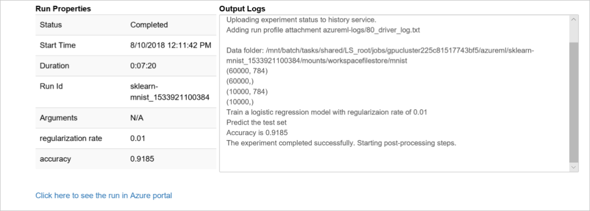
from azureml.widgets import RunDetails
RunDetails(run).show()

监控的结果如下：

显示日志

run.wait_for_completion(show_output=False)  # specify True for a verbose log

显示运行的结果

显示运行结果也非常简单:

print(run.get_metrics())

注册模型

等候训练完成了之后，我们需要将训练得到结果的模型注册到workspace里：
我们可以先显示以下模型的路径：

print(run.get_file_names())

然后注册到workspace

# register model
model = run.register_model(model_name='sklearn_mnist',
                           model_path='outputs/sklearn_mnist_model.pkl')
print(model.name, model.id, model.version, sep='\t')

至此我们完成了通过jupyter notebook 训练模型，显示测试数据，注册模型等等要素，请仔细体会一下这些要素，从这些具体的步骤中可以容易的将机器学习应用到实际的生产中。